Thanls to Dan Oehm for sharing his tips on addind icons in the script titles!

Introduction

The #TidyTuesday weekly challenge is organised by the R4DS (R for Data Science) Online Learning Community.

Every tuesday throughout the year, participants work on a common dataset and share the plots they create.

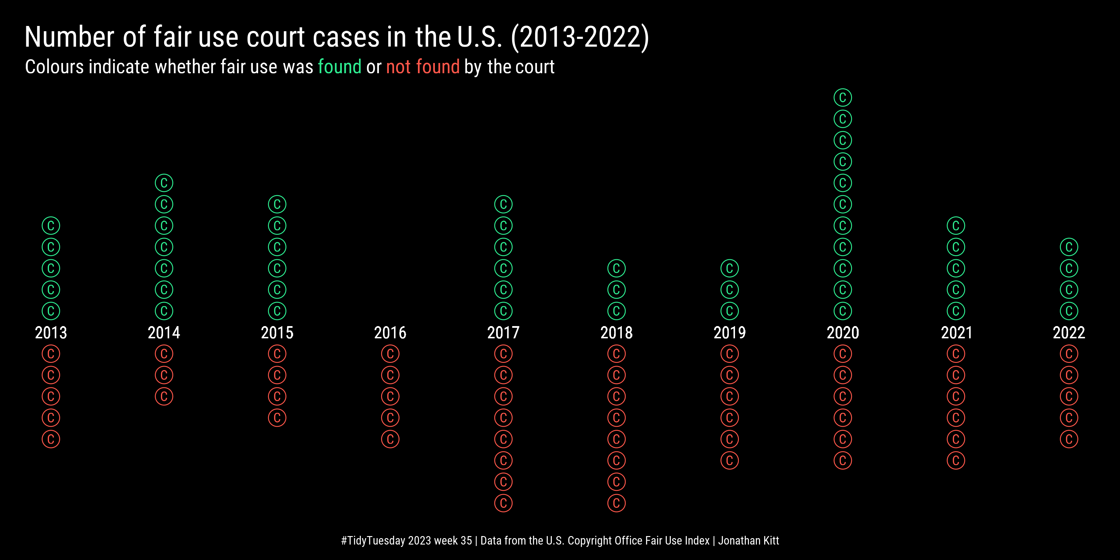
The dataset for this challenge comes from the U.S. Copyright Office Fair Use Index.

Getting the data

First of all, let’s load the packages we’ll be using :

{tidyverse} to clean the data and create the plots
{showtext} to change the fonts used
{ggtext} to use colours in the title

If you don’t have these packages installed, simply use the install.packages() function.

# 📦 Load packages ----

library(tidyverse)
library(showtext)
library(ggtext)

We also load the fonts we will use in the plots: Bebas Neue for the text and Londrina Shadow for the title.

# 🔤 Import fonts ----

font_add_google("Roboto Condensed", "Roboto Condensed")
showtext_auto()

We can now download the dataset :

# ⬇️ Import the dataset ----

fair_use_cases <- readr::read_csv("https://raw.githubusercontent.com/rfordatascience/tidytuesday/master/data/2023/2023-08-29/fair_use_cases.csv")

The dataset has 251 observations (rows) and 7 variables (columns).

Cleaning the data

We use the following code to clean the data:

# 🧹  Clean the data ----

d <- fair_use_cases |>
  # keep years 2013-2022
  filter(year >= 2013) |>
  # count number of found/not found cases per year
  count(year, fair_use_found) |>
  # repeat each row n times (n = nb of occurences)
  uncount(n) |>
  # create a row index
  mutate(case_id = 1:n(), .by = c(year, fair_use_found)) |>
  # use negative values for "not found" cases
  mutate(y = case_when(fair_use_found == TRUE ~ case_id,
                       TRUE ~ -case_id))

Creating the plot

We use the following code to create the plot:

p <- ggplot(data = d) +
  geom_point(aes(x = year, y = y,
                 colour = fair_use_found),
             shape = 21, size = 6,
             show.legend = FALSE) +
  geom_text(aes(x = year, y = y,
                colour = fair_use_found),
            label = "C",
            family = "Roboto Condensed", size = 12,
            show.legend = FALSE) +
  geom_text(aes(x = year, y = 0, label = year),
            family = "Roboto Condensed", size = 15,
            colour = "white") +
  scale_colour_manual(values = c("#fd574a", "#2eed91")) +
  labs(title = "Number of fair use court cases in the U.S. (2013-2022)",
       subtitle = "Colours indicate whether fair use was<span style='color:#2eed91;'> found</span> or <span style='color:#fd574a;'>not found</span> by the court",
       caption = "#TidyTuesday 2023 week 35 | Data from the U.S. Copyright Office Fair Use Index | Jonathan Kitt") +
  theme_void() +
  theme(panel.background = element_rect(fill = "black", colour = "black"),
        plot.background = element_rect(fill = "black", colour = "black"),
        plot.title = element_markdown(family = "Roboto Condensed",
                                      colour = "white", size = 75,
                                      margin = margin(t = 20, l = 20)),
        plot.subtitle = element_markdown(family = "Roboto Condensed",
                                         colour = "white", size = 50,
                                         margin = margin(t= 5, l = 20)),
        plot.caption = element_text(family = "Roboto Condensed",
                                    colour = "white", size = 30,
                                    hjust = 0.5, margin = margin(t = 10, b = 10)))

We now create the second plot:

# ✏️ Create the plot ----

p2 <- ggplot() +
  geom_rect(data = p2_scores,
             aes(xmin = x - 0.85, xmax = x + 0.85,
                 ymin = 0, ymax = total_thsd),
            fill = "#edeb00") +
  geom_text(data = p2_scores,
            aes(x = x, y = total_thsd - 160, label = total_thsd),
            family = "Bebas Neue", colour = "black", size = 18) +
  geom_text(data = p2_x_labels,
            aes(x = x, y = y, label = label),
            family = "Bebas Neue", colour = "white", size = 18) +
  geom_text(data = p2_text,
            aes(x = x, y = y, label = label),
            family = "Bebas Neue", colour = "white", size = 20,
            hjust = 0) +
  xlim(-1, 46) +
  theme_void() +
  theme(panel.background = element_rect(fill = "black"),
        plot.background = element_rect(fill = "black"))

# 💾 Export plot ----

ggsave("figs/tt_2023_w35_fair_use.png", p, dpi = 320, width = 12, height = 6)

And here’s the result!