Introduction

The #TidyTuesday weekly challenge is organised by the R4DS (R for Data Science) Online Learning Community.

Every tuesday throughout the year, participants work on a common dataset and share the plots they create.

The dataset for this challenge comes from Wikipedia articles.

Getting the data

First of all, let’s load the packages we’ll be using :

{tidyverse} to clean the data and create the plots
{showtext} to change the fonts used
{rgdal} and {rgeos} to plot the U.S. states as hexagons
{ggtext} to add colours in the plot title

If you don’t have these packages installed, simply use the install.packages() function.

# Load the packages
library(tidyverse)
library(showtext)
library(rgdal)
library(rgeos)
library(ggtext)

We also load the fonts we will use in the plots: Roboto Condensed for the text and Bangers for the title.

# Import the fonts
font_add_google("Roboto Condensed", "Roboto Condensed")
font_add_google("Bangers", "Bangers")
showtext_auto()

We can now download the dataset :

# Download the dataset
states <- read_csv('https://raw.githubusercontent.com/rfordatascience/tidytuesday/master/data/2023/2023-08-01/states.csv')

We also download the data to plot U.S. states as hexagons here. We save the GEO JSON file in a raw/ directory.

We then load the data:

# Download the dataset
us_hex <- readOGR("raw/us_states_hexgrid.geojson")

For a quick overview of the data, we use the glimpse() function from the {dplyr} package:

# Explore the dataset
glimpse(states)

Rows: 50
Columns: 14
$ state               <chr> "Alabama", "Alaska", "Arizona", "Arkansas", "Calif…
$ postal_abbreviation <chr> "AL", "AK", "AZ", "AR", "CA", "CO", "CT", "DE", "F…
$ capital_city        <chr> "Montgomery", "Juneau", "Phoenix", "Little Rock", …
$ largest_city        <chr> "Huntsville", "Anchorage", "Phoenix", "Little Rock…
$ admission           <date> 1819-12-14, 1959-01-03, 1912-02-14, 1836-06-15, 1…
$ population_2020     <dbl> 5024279, 733391, 7151502, 3011524, 39538223, 57737…
$ total_area_mi2      <dbl> 52420, 665384, 113990, 53179, 163695, 104094, 5543…
$ total_area_km2      <dbl> 135767, 1723337, 295234, 137732, 423967, 269601, 1…
$ land_area_mi2       <dbl> 50645, 570641, 113594, 52035, 155779, 103642, 4842…
$ land_area_km2       <dbl> 131171, 1477953, 294207, 134771, 403466, 268431, 1…
$ water_area_mi2      <dbl> 1775, 94743, 396, 1143, 7916, 452, 701, 540, 12133…
$ water_area_km2      <dbl> 4597, 245384, 1026, 2961, 20501, 1170, 1816, 1399,…
$ n_representatives   <dbl> 7, 1, 9, 4, 52, 8, 5, 1, 28, 14, 2, 2, 17, 9, 4, 4…
$ demonym             <chr> "Alabamian", "Alaskan", "Arizonan", "Arkansan", "C…

The dataset has 50 observations (rows) and 14 variables (columns).

Each row represents one U.S. states.

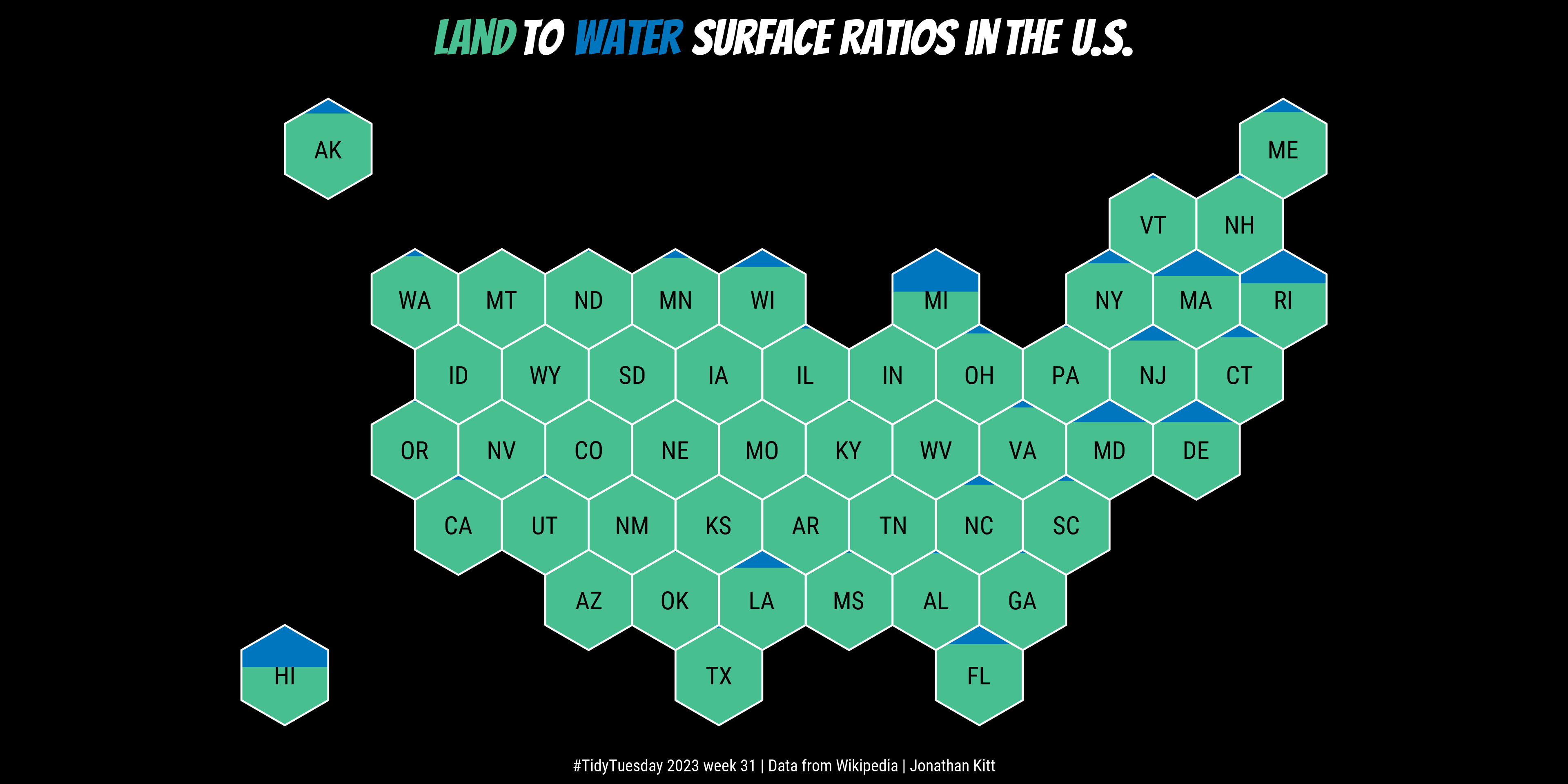
We’re going to represent the ratios between land and water surfaces for each state.

Cleaning the data

We use the following code to calculate the land/water ratios:

# Land to water area ratios
land_to_water_ratios <- states |>
  # calculate land/total and water/total area ratios
  mutate(land_area_ratio = round(land_area_km2 / total_area_km2, 3),
         water_area_ratio = round(1 - land_area_ratio, 3)) |>
  # select columns
  select(id = postal_abbreviation, state, land_area_ratio, water_area_ratio)

# View first lines of cleaned data
head(land_to_water_ratios)

# A tibble: 6 × 4
  id    state      land_area_ratio water_area_ratio
  <chr> <chr>                <dbl>            <dbl>
1 AL    Alabama              0.966            0.034
2 AK    Alaska               0.858            0.142
3 AZ    Arizona              0.997            0.003
4 AR    Arkansas             0.979            0.021
5 CA    California           0.952            0.048
6 CO    Colorado             0.996            0.004

We calculate the coordinates for boundaries between land and water surfaces for each hexagon:

# Prepare data to create hex map of land to water ratio per US state
us_clean <- us_hex |>
  # transform hex data into table
  fortify(region = "iso3166_2") |>
  # transform into tibble format
  as_tibble() |>
  # select columns
  select(id, long, lat) |>
  # join land to water ratios values
  left_join(land_to_water_ratios) |>
  # remove District of Columbia
  filter(id != "DC") |>
  # add column with point order
  mutate(pt_nb = rep(1:7, times = 50), .before = long) |>
  # group by state id
  group_by(id) |>
  # calculate parameters for each state
  mutate(
    # total area for reactangle around hex
    area_rect = (long[pt_nb == 3] - long[pt_nb == 5]) * (lat[pt_nb == 1] - lat[pt_nb == 4]),
    # slope of upper hex triangle
    slope = (lat[pt_nb == 6] - lat[pt_nb == 1]) / (long[pt_nb == 6] - long[pt_nb == 1]),
    # y coordinate for horizontal border btwn land/water
    split_y = ((land_area_ratio * area_rect) / (long[pt_nb == 2] - long[pt_nb == 6]) + lat[pt_nb == 4]),
    # determine type of split : 1 if split line below upper triangle / 2 if not
    split_type = case_when(split_y <= lat[pt_nb == 2] ~ 1, TRUE ~ 2),
    # calculate x coordinates for horizontal border btwn land/water
    split_x1 = case_when(split_type == 1 ~ min(long),
                         split_type == 2 ~ long[pt_nb == 6] + ((split_y - lat[pt_nb == 6]) / slope)),
    split_x2 = case_when(split_type == 1 ~ max(long),
                         split_type == 2 ~ long[pt_nb == 1] + (long[pt_nb == 1] - split_x1))
    )

# Subset us_clean data for type 1 split
us_clean_type1 <- us_clean |>
  # filter data
  filter(split_type == 1) |>
  # create new columns to keep points needed for plot
  mutate(pt1_x = long[pt_nb == 1], pt1_y = lat[pt_nb == 1],
         pt2_x = long[pt_nb == 2], pt2_y = lat[pt_nb == 2],
         pt3_x = unique(split_x2), pt3_y = unique(split_y),
         pt4_x = unique(split_x1), pt4_y = unique(split_y),
         pt5_x = long[pt_nb == 6], pt5_y = lat[pt_nb == 6],
         pt6_x = pt1_x, pt6_y = pt1_y) |>
  # select columns
  select(id, pt1_x:pt6_y) |>
  # ungroup data
  ungroup() |>
  # pivot to long format
  pivot_longer(cols = -id, names_to = "pt", values_to = "value") |>
  # separate "pt" column
  separate(col = pt, into = c("pt_nb", "xy"), sep = "_") |>
  # remove "pt" string from pt_nb column
  mutate(pt_nb = str_remove_all(pt_nb, "pt")) |>
  # keep distinct rows
  distinct() |>
  # pivot to wide format
  pivot_wider(id_cols = id:pt_nb, names_from = "xy", values_from = "value")

# Subset us_clean data for type 2 split
us_clean_type2 <- us_clean |>
  # filter data
  filter(split_type == 2) |>
  # create new columns to keep points needed for plot
  mutate(pt1_x = long[pt_nb == 1], pt1_y = lat[pt_nb == 1],
         pt2_x = unique(split_x2), pt2_y = unique(split_y),
         pt3_x = unique(split_x1), pt3_y = unique(split_y),
         pt4_x = pt1_x, pt4_y = pt1_y) |>
  # select columns
  select(id, pt1_x:pt4_y) |>
  # ungroup data
  ungroup() |>
  # pivot to long format
  pivot_longer(cols = -id, names_to = "pt", values_to = "value") |>
  # separate "pt" column
  separate(col = pt, into = c("pt_nb", "xy"), sep = "_") |>
  # remove "pt" string from pt_nb column
  mutate(pt_nb = str_remove_all(pt_nb, "pt")) |>
  # keep distinct rows
  distinct() |>
  # pivot to wide format
  pivot_wider(id_cols = id:pt_nb, names_from = "xy", values_from = "value")

We calculate the coordinates of each hexagon’s centre to add text labels:

# Calculate centres of polygons to plot state labels
centres <- gCentroid(us_hex, byid = TRUE) |>
  as_tibble()

labels <- us_hex@data$iso3166_2

hex_labels <- tibble(id = labels,
                     centres) |>
  filter(id != "DC")

# Clean global environment
rm(centres, labels, land_to_water_ratios, states, us_hex)

Creating the plot

p <- ggplot() +
  geom_polygon(data = us_clean, aes(x = long, y = lat, group = id),
               colour = NA, fill = "#48bf91") +
  geom_polygon(data = us_clean_type1, aes(x = x, y = y, group = id),
               colour = NA, fill = "#0076be") +
  geom_polygon(data = us_clean_type2, aes(x = x, y = y, group = id),
               colour = NA, fill = "#0076be") +
  geom_polygon(data = us_clean, aes(x = long, y = lat, group = id),
               colour = "white", fill = NA, linewidth = 0.5) +
  geom_text(data = hex_labels, aes(x = x, y = y, label = id),
            family = "Roboto Condensed", colour = "black", size = 16) +
  coord_map() +
  labs(title = "<span style='color:#48bf91;'>Land</span> to <span style='color:#0076be;'>water</span> surface ratios in the U.S.",
       caption = "#TidyTuesday 2023 week 31 | Data from Wikipedia | Jonathan Kitt") +
  theme_void() +
  theme(panel.background = element_rect(fill = "black", colour = NA),
        plot.background = element_rect(fill = "black", colour = NA),
        plot.title = element_markdown(family = "Bangers", size = 90,
                                      hjust = 0.5, colour = "white",
                                      margin = margin(t = 20)),
        plot.caption = element_text(family = "Roboto Condensed", colour = "white", size = 30,
                                    hjust = 0.5, 
                                    margin = margin(b = 5)))

ggsave("figs/tt_2023_w31_us.png", p, dpi = 320, width = 12, height = 6)

And here’s the result!